こんにちは、@Yoshimiです。
機械学習のチュートリアルでデータセットを使うことも多いはずです。今回はIrisのデータセットの中身・構造を確認したいと思います。
Irisデータセット
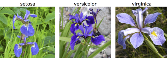
Irisデータセットはアヤメの種類と特徴量に関するデータセットで、3種類のアヤメの花弁と萼に関する特徴量について多数のデータを提供しています。
早速中身を確認していきましょう。
データの取得
sklearnのdatasetsを読み込んでload_iris()で取得可能です。
from sklearn.datasets import load_iris

iris_dataset = load_iris()

for key, value in zip(iris_dataset.keys(), iris_dataset.values()):
    print("{}:\n{}\n".format(key, value))
データの構造は辞書方です。150個体のアヤメに関する特徴量の配列と種類、名称が格納されています。
[[5.1 3.5 1.4 0.2] [4.9 3. 1.4 0.2] [4.7 3.2 1.3 0.2] –(中略)–
[6.5 3. 5.2 2. ] [6.2 3.4 5.4 2.3] [5.9 3. 5.1 1.8]]
target:
[0 0 0 0 0 0 0 0 0 0 0 0 0 0 0 0 0 0 0 0 0 0 0 0 0 0 0 0 0 0 0 0 0 0 0 0 0
0 0 0 0 0 0 0 0 0 0 0 0 0 1 1 1 1 1 1 1 1 1 1 1 1 1 1 1 1 1 1 1 1 1 1 1 1
1 1 1 1 1 1 1 1 1 1 1 1 1 1 1 1 1 1 1 1 1 1 1 1 1 1 2 2 2 2 2 2 2 2 2 2 2
2 2 2 2 2 2 2 2 2 2 2 2 2 2 2 2 2 2 2 2 2 2 2 2 2 2 2 2 2 2 2 2 2 2 2 2 2
2 2]
target_names:
[‘setosa’ ‘versicolor’ ‘virginica’]
DESCR:
.. _iris_dataset:
Iris plants dataset
——————–
**Data Set Characteristics:**
:Number of Instances: 150 (50 in each of three classes)
:Number of Attributes: 4 numeric, predictive attributes and the class
:Attribute Information:
– sepal length in cm
– sepal width in cm
– petal length in cm
– petal width in cm
– class:
– Iris-Setosa
– Iris-Versicolour
– Iris-Virginica
:Summary Statistics:
============== ==== ==== ======= ===== ====================
Min Max Mean SD Class Correlation
============== ==== ==== ======= ===== ====================
sepal length: 4.3 7.9 5.84 0.83 0.7826
sepal width: 2.0 4.4 3.05 0.43 -0.4194
petal length: 1.0 6.9 3.76 1.76 0.9490 (high!)
petal width: 0.1 2.5 1.20 0.76 0.9565 (high!)
============== ==== ==== ======= ===== ====================
:Missing Attribute Values: None
:Class Distribution: 33.3% for each of 3 classes.
:Creator: R.A. Fisher
:Donor: Michael Marshall (MARSHALL%PLU@io.arc.nasa.gov)
:Date: July, 1988
The famous Iris database, first used by Sir R.A. Fisher. The dataset is taken
from Fisher’s paper. Note that it’s the same as in R, but not as in the UCI
Machine Learning Repository, which has two wrong data points.
This is perhaps the best known database to be found in the
pattern recognition literature. Fisher’s paper is a classic in the field and
is referenced frequently to this day. (See Duda & Hart, for example.) The
data set contains 3 classes of 50 instances each, where each class refers to a
type of iris plant. One class is linearly separable from the other 2; the
latter are NOT linearly separable from each other.
.. topic:: References
– Fisher, R.A. “The use of multiple measurements in taxonomic problems”
Annual Eugenics, 7, Part II, 179-188 (1936); also in “Contributions to
Mathematical Statistics” (John Wiley, NY, 1950).
– Duda, R.O., & Hart, P.E. (1973) Pattern Classification and Scene Analysis.
(Q327.D83) John Wiley & Sons. ISBN 0-471-22361-1. See page 218.
– Dasarathy, B.V. (1980) “Nosing Around the Neighborhood: A New System
Structure and Classification Rule for Recognition in Partially Exposed
Environments”. IEEE Transactions on Pattern Analysis and Machine
Intelligence, Vol. PAMI-2, No. 1, 67-71.
– Gates, G.W. (1972) “The Reduced Nearest Neighbor Rule”. IEEE Transactions
on Information Theory, May 1972, 431-433.
– See also: 1988 MLC Proceedings, 54-64. Cheeseman et al”s AUTOCLASS II
conceptual clustering system finds 3 classes in the data.
– Many, many more …
feature_names:
[‘sepal length (cm)’, ‘sepal width (cm)’, ‘petal length (cm)’, ‘petal width (cm)’]
filename:
/opt/anaconda3/lib/python3.7/site-packages/sklearn/datasets/data/iris.csv
データのキーは以下の通りです。
from sklearn.datasets import load_iris

iris_dataset = load_iris()

print(iris_dataset.keys())
データの内容
'data':特徴量のデータセット
150個体のアヤメに関する、4つの特徴量をレコードとしたデータセット。列のインデックス(0,1,2,3)が4つの特徴量に対応しています。
[4.9, 3. , 1.4, 0.2],
[4.7, 3.2, 1.3, 0.2],
[4.6, 3.1, 1.5, 0.2],
[5. , 3.6, 1.4, 0.2],
…..
[6.7, 3. , 5.2, 2.3],
[6.3, 2.5, 5. , 1.9],
[6.5, 3. , 5.2, 2. ],
[6.2, 3.4, 5.4, 2.3],
[5.9, 3. , 5.1, 1.8]])
'target':アヤメの種類に対応したコード
3種類のアヤメに対応した0~2のコードの配列です。150個体のアヤメに対応した1次元配列です。
0, 0, 0, 0, 0, 0, 0, 0, 0, 0, 0, 0, 0, 0, 0, 0, 0, 0, 0, 0, 0, 0,
0, 0, 0, 0, 0, 0, 1, 1, 1, 1, 1, 1, 1, 1, 1, 1, 1, 1, 1, 1, 1, 1,
1, 1, 1, 1, 1, 1, 1, 1, 1, 1, 1, 1, 1, 1, 1, 1, 1, 1, 1, 1, 1, 1,
1, 1, 1, 1, 1, 1, 1, 1, 1, 1, 1, 1, 2, 2, 2, 2, 2, 2, 2, 2, 2, 2,
2, 2, 2, 2, 2, 2, 2, 2, 2, 2, 2, 2, 2, 2, 2, 2, 2, 2, 2, 2, 2, 2,
2, 2, 2, 2, 2, 2, 2, 2, 2, 2, 2, 2, 2, 2, 2, 2, 2, 2])
'target_names':アヤメの種類名
アヤメの3つの種類の種類名です。
- setosa:0
- versicolor:1
- virginica:2
に対応しています。
'feature_names':特徴名
アヤメの種類のクラス分けに使う4つの特徴。
- ‘sepal length (cm)’ 萼の長さ:0
- ‘sepal width (cm)’ 萼の幅:1
- ‘petal length (cm)’ 花弁の長さ:2
- ‘petal width (cm)’ 花弁の幅:3
'filename':ファイル名
CSVファイルの位置が示されています。このデータは辞書方とは違い、1行目にデータ数(150)、特徴量数、特徴量名称が並んでおり、その後に150個体のアヤメのデータが並んでいます。データフレームとして確認したい場合はこの情報が見やすいです。ただし、feature_namesやDESCRにあたるデータは格納されていないので、ご注意を。
'DESCR':データセットの説明
データの説明がびっしり書いてあります。
.. _iris_dataset:
・
・
・以下
最後に
Irisデータセットに限らず、scikit-learnには様々なデータセットがあります。実務で使うには整いすぎているので、チュートリアル的に利用するのが良いです。
しかし、検証するには非常に使いやすい(前処理をする必要がないので)データです。アルゴリズムチェックなどで積極的に使っていきましょう。
なりたい自分になれる
スキルアップならUdemy
私も利用し、高収入エンジニアになったのよ。未経験から機械学習、データサイエンティスト、アプリ開発エンジニアを目指せるコンテンツが多数あります。優秀な講師が多数!割引を利用すれば1,200円〜から動画購入可能です。!